【零基础学绘图】之绘制venn图（五）

venn图是R的基础绘图之一，方法非常简单易学，网络上也有较多的教程和在线venn图绘制。这里我们简单讲一下从原始数据开始是如何一步一步绘图的，包含数据读写、数据处理和绘图。

文章导读

一、数据处理

1. otu文件、分组文件查看

2. 从OTU文件中将属于同一组的样品数据提出，并求和

3. 统计不同分组的OTU个数

二、venn图绘制

1. 安装和加载VennDiagram

2. 绘图

三、超过5组的花瓣图绘制（Flower plots）

1. 花瓣图绘制

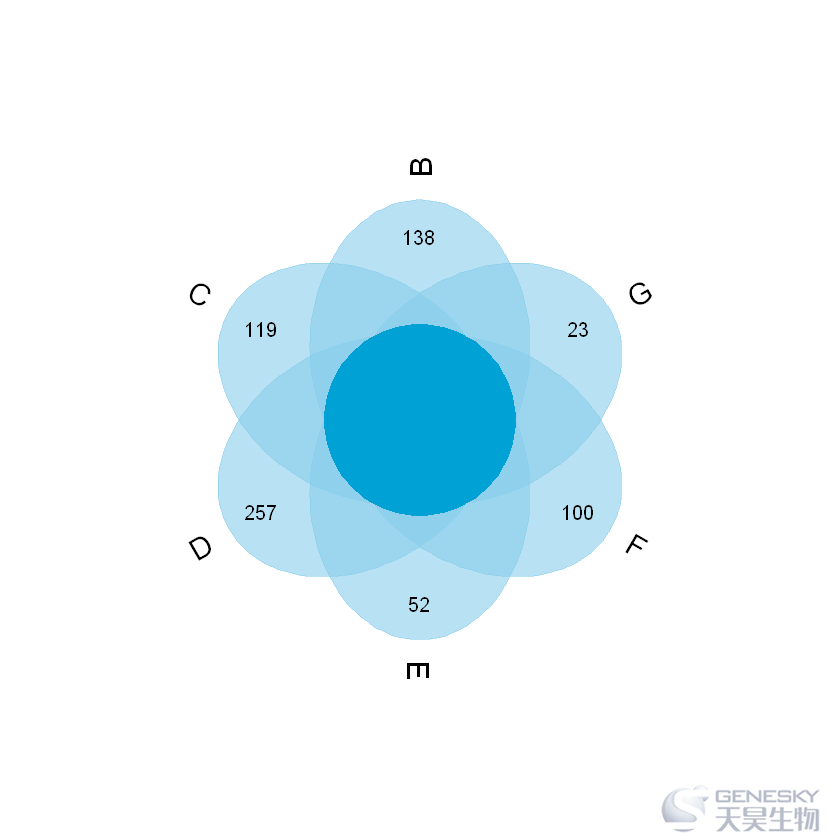
    2. 调整短轴和长轴的参数

一

数据处理

1.otu文件、分组文件查看
In [1]:
df = read.table('otu.tax.0.03.xls',header = T,check.names = F,sep = ' ', row.names = 1,quote = '',comment.char = '')
head(df,3)

Out[1]:
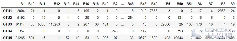
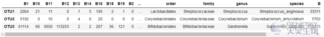
B1 B10 B11 B12 B13 B14 B16 B18 B19 B2 ... F9 OTUsize Taxonomy superkingdom phylum class order family genus species
OTU1 2004 21 11 0 1 3 195 2 1 0 ... 0 195460 Bacteria{superkingdom}(100);Firmicutes{phylum}(100);Bacilli{class}(100);Lactobacillales{order}(100);Streptococcaceae{family}(100);Streptococcus{genus}(100);Streptococcus_anginosus{species}(100) Bacteria Firmicutes Bacilli Lactobacillales Streptococcaceae Streptococcus Streptococcus_anginosus
OTU2 5192 0 10 0 4 0 20 0 0 0 ... 0 5844 Bacteria{superkingdom}(100);Actinobacteria{phylum}(100);Actinobacteria{class}(100);Corynebacteriales{order}(100);Corynebacteriaceae{family}(100);Corynebacterium{genus}(100);Corynebacterium_amycolatum{species}(83) Bacteria Actinobacteria Actinobacteria Corynebacteriales Corynebacteriaceae Corynebacterium Corynebacterium_amycolatum
OTU3 61114 66 5850 113253 2 2 207 36 121 0 ... 0 804859 Bacteria{superkingdom}(100);Actinobacteria{phylum}(100);Actinobacteria{class}(100);Bifidobacteriales{order}(100);Bifidobacteriaceae{family}(100);Gardnerella{genus}(100);Gardnerella_vaginalis{species}(100) Bacteria Actinobacteria Actinobacteria Bifidobacteriales Bifidobacteriaceae Gardnerella Gardnerella_vaginalis

In [2]:
info = read.table('sample_group.txt')
head(info,5)

Out[2]:
V1 V2
B1 BB 10 BB 11 BB 12 BB 13 B

In [3]:
group=info$V2

levels(group)

Out[3]:
'B' 'C' 'D' 'E' 'F' 'G'

2.从OTU文件中将属于同一组的样品数据提出，并求和

In [4]:
info[info$V2=='B','V1']

Out[4]:
B1 B10 B11 B12 B13 B14 B16 B18 B19 B2 B22 B23 B26 B27 B28 B3 B4 B41 B45 B46 B49 B5 B50 B51 B6 B7 B8 B9

In [5]:
head(df[,info[info$V2=='B','V1']],5)

Out[5]:

In [6]:
df$B = apply(df[,info[info$V2=='B','V1']],1,sum)
df$C = apply(df[,info[info$V2=='C','V1']],1,sum)
df$D = apply(df[,info[info$V2=='D','V1']],1,sum)
df$E = apply(df[,info[info$V2=='E','V1']],1,sum)
df$F = apply(df[,info[info$V2=='F','V1']],1,sum)
df$G = apply(df[,info[info$V2=='G','V1']],1,sum)

In [7]:
head(df,3)

Out[7]:

3.统计不同分组的OTU个数

In [8]:
length(rownames(df)[df$B!=0])

Out[8]:
1370

In [9]:
length(rownames(df)[df$C!=0])

Out[9]:
894

In [10]:
length(rownames(df)[df$D!=0])

Out[10]:
1630

In [11]:
length(rownames(df)[df$E!=0])

Out[11]:
855

In [12]:
length(rownames(df)[df$F!=0])

Out[12]:
684

In [13]:
length(rownames(df)[df$G!=0])

Out[13]:
473

二

venn图绘制

1.安装和加载VennDiagram

In [14]:
install.packages('VennDiagram')

In [15]:
library(VennDiagram)

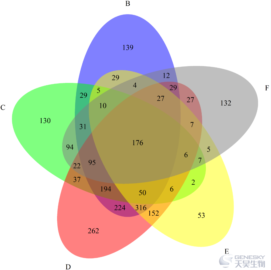
2.绘图

In [16]:
x= list(B=rownames(df)[df$B!=0],
C=rownames(df)[df$C!=0],
D=rownames(df)[df$D!=0], E=rownames(df)[df$E!=0],
F=rownames(df)[df$F!=0])

venn.diagram(x,filename = 'venn_5set.png',col='transparent',fill=c('blue','green','red','yellow','grey50'))

Out[16]:

In [17]:
x= list(B=rownames(df)[df$B!=0],

     

								   C=rownames(df)[df$C!=0],

     

								   D=rownames(df)[df$D!=0],

     

								   E=rownames(df)[df$E!=0])

venn.diagram(x,filename = 'venn_4set.png',col='transparent',fill=c('blue','green','red','yellow'))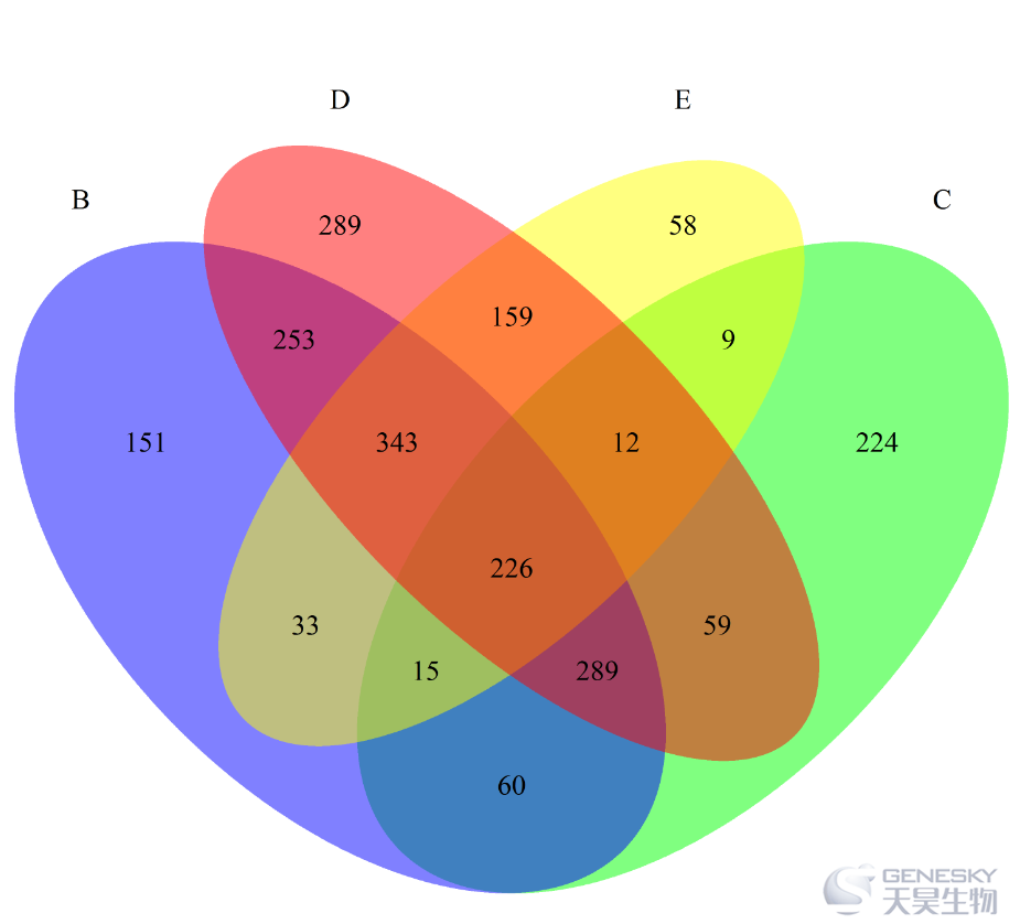

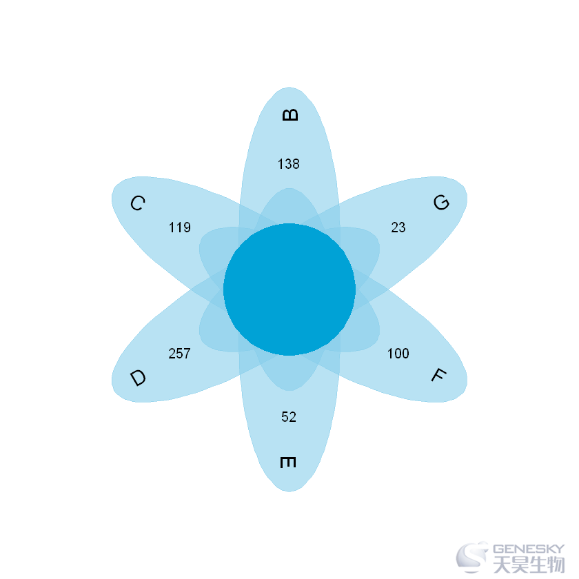
Out[17]:

3.检验数值是否正确

In [18]:
length(rownames(df)[df$B!=0 & df$C==0 & df$D==0 & df$E==0 & df$F==0 ])

Out[18]:
139

In [19]:
length(rownames(df)[df$B!=0 & df$C!=0 & df$D!=0 & df$E!=0 & df$F!=0 ])

Out[19]:
176

In [20]:

length(rownames(df)[df$B!=0 & df$C==0 & df$D!=0 & df$E==0 & df$F==0])

Out[20]:
224

仅B组存在的个数为139，B、C、D、E、F共有的个数是176，均与5组venn图中的数值一致。

三

超过5组的花瓣图绘制

（Flower plots）

1.花瓣图绘制
In [21]:
install.packages('plotrix')
library(plotrix)

In [22]:
flower_plot <- function(sample, value, start, a, b,

 

								  ellipse_col = rgb(135, 206, 235, 150, max = 255),

 

								  circle_col = rgb(0, 162, 214, max = 255),

 

								  circle_text_cex = 1.5

) {

  

								  par( bty = "n", ann = F, xaxt = "n", yaxt = "n", mar = c(1,1,1,1))

  

								  plot(c(0,10),c(0,10),type="n")

  

								  n   <- length(sample)

  

								  deg <- 360 / n

  

								  res <- lapply(1:n, function(t){

   

								   draw.ellipse(x = 5 + cos((start + deg * (t - 1)) * pi / 180),

              

								      y = 5 + sin((start + deg * (t - 1)) * pi / 180),

              

								      col = ellipse_col,

              

								      border = ellipse_col,

              

								      a = a, b = b, angle = deg * (t - 1))

   

								   text(x = 5 + 2.5 * cos((start + deg * (t - 1)) * pi / 180),

      

								    y = 5 + 2.5 * sin((start + deg * (t - 1)) * pi / 180),

      

								    value[t]

     

								    )

								   if (deg * (t - 1) < 180 && deg * (t - 1) > 0 ) {     

								    text(x = 5 + 3.3 * cos((start + deg * (t - 1)) * pi / 180),        

								    y = 5 + 3.3 * sin((start + deg * (t - 1)) * pi / 180),        

								    sample[t],        

								    srt = deg * (t - 1) - start,        

								    adj = 1,        

								    cex = circle_text_cex       

								    )

								   } else {     

								     text(x = 5 + 3.3 * cos((start + deg * (t - 1)) * pi / 180),        

								     y = 5 + 3.3 * sin((start + deg * (t - 1)) * pi / 180),        

								     sample[t],        

								     srt = deg * (t - 1) + start,        

								     adj = 0,        

								     cex = circle_text_cex       

								    )   

								   }       

								  }) 

								  draw.circle(x = 5, y = 5, r = 1.3, col = circle_col, border = circle_col)

								}

第一个参数sample为样本名字构成的向量，第二个参数valus为每个样本对应的值，第三个参数start为起始椭圆的角度，第四个参数a为椭圆的短轴的长度，第五个参数b为椭圆的长轴的长度。

计算每组特有的OTU数目
In [23]:
b=length(rownames(df)[df$B!=0 & df$C==0 & df$D==0 & df$E==0 & df$F==0 & df$G==0 ])
c=length(rownames(df)[df$B==0 & df$C!=0 & df$D==0 & df$E==0 & df$F==0 & df$G==0 ])
d=length(rownames(df)[df$B==0 & df$C==0 & df$D!=0 & df$E==0 & df$F==0 & df$G==0 ])
e=length(rownames(df)[df$B==0 & df$C==0 & df$D==0 & df$E!=0 & df$F==0 & df$G==0 ])
f=length(rownames(df)[df$B==0 & df$C==0 & df$D==0 & df$E==0 & df$F!=0 & df$G==0 ])
g=length(rownames(df)[df$B==0 & df$C==0 & df$D==0 & df$E==0 & df$F==0 & df$G!=0 ])

绘制花瓣图
In [24]:
flower_plot(c('B','C','D','E','F','G'),c(b,c,d,e,f,g), 90,1,3)

Out[24]: